Plot Page - Fit Plots

The fit plot properties Plot page contains the options to change the data and plot intervals, the number of points, and to generate statistics for the fit curve. To view and edit fit plot properties, click on the fit plot in the plot window or Object Manager to select it. Then, click on the Plot tab in the Property Manager.

The fit properties are displayed in the Property Manager on the Plot tab.

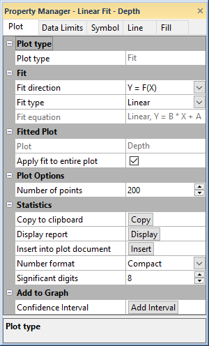
Plot Type

The Plot type property displays the type of plot.

Fit

The Fit section displays the fit curve equation and includes a Function button for editing the fit curve when a custom fit curve is selected.

Fit Direction

The Fit direction property sets whether the fit is added where Y is a function of X (Y=F(X)) or where X is a function of Y (X=F(Y)). The Fit direction property is not available for custom fit curves. Custom fit curves must be Y as a function of X.

Fit Type

Select the fit equation you wish to use in the Fit type list. Select one of the many predefined fit types or select a previously created custom fit. Click the Define Custom Fit command to create a new custom fit equation.

Fit Equation

The selected fit curve equation is displayed in the Fit equation box. This is the equation for the existing fit curve. When a predefined fit equation is selected in the Fit type field, the Fit equation is read-only information. When a custom fit equation is selected in the Fit type field, the Fit equation becomes editable and the Name, Remove from fit types, and Parameters properties are available.

Custom Fit Equation

When a custom fit equation is selected in the Fit type field, you can edit the custom fit curve equation in the Fit equation field. Type in the Fit equation field to edit the custom fit equation. Click the Function button to insert predefined mathematical functions into the fit equation.

Name

When a custom fit equation is selected in the Fit type list, the Name property is available. The custom fit name is displayed in the Name field. You can edit the Name if desired.

Remove Fit from Types

Click Remove to remove the custom fit from this and all future Fit type lists. When the custom fit is removed, the Fit type becomes Linear.

Parameters

The Parameters section includes properties for improving or limiting the custom fit parameter values. By default, the initial guess is 1 and parameters are able to vary across the largest possible range, -1.79769x10308 to 1.79769x10308.

Select which parameter you wish to edit in the Parameter list. The selected Parameter initial guess, minimum, and maximum values are displayed.

Specify an initial guess for the parameter value in the Initial value field if you can. This is useful for ensuring Grapher finds the global best fit when the Fit equation is susceptible to local best fit values.

Specify the Minimum value for the Parameter if the parameter value should have a lower bound. For example, if the parameter in your custom fit equation cannot be negative, set the Minimum to 0.

Specify the Maximum value for the Parameter if the parameter value should have an upper bound. For example, if you know your parameter value cannot exceed 100, then type 100 in the Maximum field.

Fitted Plot

The Fitted Plot section defines the plot being fitted and which data in the plot should be fitted.

Plot

The Plot property displays the plot to which the fit is applied. This value is informational and cannot be changed.

Apply Fit to Entire Plot

The Apply fit to entire plot option uses all of the plot's data to determine the fit. Select the Apply fit to entire plot option to automatically set the Minimum plot value to fit and Maximum plot value to fit to the minimum and maximum extents of the plot. Clear the Apply fit to entire plot to specify a subset of the plot's data to fit.

When a single class is selected, Apply fit to entire plot will not force Grapher to fit data outside the selected class. Therefore, the fit curve statistics will not change. This can be used to quickly toggle between drawing the fit curve across the entire plot or only along the extents of the class. Typically, the Data Limits page is used to change where a plot is drawn.

Minimum and Maximum Plot Value to Fit

After the Apply fit to entire plot check box is cleared, the Minimum plot value to fit and Maximum plot value to fit properties are available. Specify a subset of the plot data to fit by typing values in the Minimum plot value to fit and Maximum plot value to fit fields. Minimum date/time and Maximum date/time options are available if the appropriate data is formatted as date/time in the worksheet.

Class

A fit curve can be calculated for a specific class in a class plot. When a fit is added to a class plot, the Class property is available in the fit curve properties. To calculate the fit for only a single class, select the desired class in the Class list. To calculate the fit for all data, select (All).

Running Average, Weighted Average, and Spline Smoothing fit curves cannot be added to class plots.

Plot Options

Some fit curves have specific options available to set. Spline smoothing, polynomial, orthogonal polynomial, running average, weighted average, LOESS, lognormal distribution, exponential PDF distribution, power PDF distribution, and inverse Gaussian distribution fits have options. All fits except weighted average and running average include the Number of points option.

Spline Smoothing

The Spline smoothing fit curve has a Spline tension factor option. The Spline tension factor value ranges from 1 to 50. Higher Spline tension factor values result in straighter lines between the data points. Lower Spline tension factor values result in more curvature to the fit line.

Polynomial and Orthogonal Polynomial

The Polynomial and Orthogonal polynomial fit curves have a Polynomial degree option. The Polynomial degree value ranges from 0 to 10. The default Polynomial degree is calculated based on the fitted data. A polynomial degree of zero is the average Y value. When the Polynomial degree value is one, the fit curve is a linear fit. Degree two is a quadratic fit, degree three is a cubic fit, and degree four is a quadric fit.

Running Average and Weighted Average

The Running average and Weighted average fit curves have a Window width option. The Windows width controls how many points are included when calculating the fit curve value at each data point. This number must be an odd number between 3 and 1001 for Running average fits and between 3 and 49 for Weighted average fits. The default window width of five averages the data point with the two values above the data point and the two values below the data point. An average of all five values is plotted as the point on the fit line. The fit is a line connecting these average points at each X data value.

The Weighted average fit curve also has a Weights section. The weights for the window can be set by expanding the Weights section and typing values for the Order properties. For example, if you have three points and want the middle point to have twice the weight of the other points, you would enter 1 for the weight of Order 1, 2 for the weight of Order 2, and 1 for the weight of Order 3. You can save the weights to a file by clicking Save in the Save weights field. Load weights from a file by clicking Load in the Load weights field. Orders are added or removed from the top and bottom of the weights list.

LOESS (LOWESS)

The LOESS (LOWESS) fit is defined by the Span, Family, and Degree. The Span is the proportion of the data used to fit the local polynomial at each point. The Span can vary between 0.1 (10%) and 1.0 (100%) of the data. Typically values between 0.25 and 0.5 are appropriate for the Span parameter. The Span is sometimes referred to as the smoothing parameter. The Family option determines the fit algorithm. When Family is set to Gaussian, a least squares fit is used. A redescending M estimator with Tukey's biweight or bisquare function is used to fit the data when Family is set to Symmetric. The Degree specifies the order of the local polynomials fit to each subset of the data. A Degree of 1 (Linear) fits a linear function to each data subset. A Degree of 2 (Quadratic) fits a quadratic function to each data subset.

Lognormal

The Lognormal fit curve has a Location value and Scale value option. The values can be any number. Click on the word Custom and select Auto box to return the values to the defaults.

Exponential PDF

The Exponential PDF fit curve has a Scale value option. The values can be any number. Click the word Custom and select Auto box to return the values to the defaults.

Power PDF

The Power PDF fit curve has a Location value and Shape value option. The values can be any number. Click the word Custom and select Auto box to return the values to the defaults.

Inverse Gaussian

The Inverse Gaussian fit curve has a Location value and Shape value option. The values can be any number. Click the word Custom and select Auto box to return the values to the defaults.

Number of Points

The Number of points option controls the number of data points used to draw the fit curve. A higher number of points result in a smoother line. A higher number of points will also take longer to generate the fit curve and update the graph. Regardless of how many points are used to draw the fit curve, all data points in the original plot inside the Plot interval are used to calculate the fit curve.

The Number of points can be any number between 2 and 2.14748e+9. The Number of points option is not available for running average and weighted average fit curves.

3D Settings

The 3D Settings section is displayed for fit plots in the 3D graphs.

Position

The Position option controls the location of the plot on the depth axis of the 3D plot. For example, 0 percent places the plot at the front of the graph, 100 percent places the plot at the back of the graph, and 50 percent places the plot in the middle of the graph.

Width

The Plot width controls the width of the plot. Plots can be 0.01 to 6 inches (0.025 and 15.24 cm) wide.

Line Frequency

Use the Line frequency field to control the cross lines along the plot width. The lines are usually drawn at each data point over the width of the plot, that is Line frequency is set to 1. When there are many points on the graph, the line color may overwrite most of the ribbon fill color. Use the Line frequency option to skip lines on the plot. For example, if Line frequency is set to 5, every fifth line is plotted on the plot. To remove all of the lines, set the Line frequency to a number greater than the total number of data points. Up to 10,000 points may be skipped between lines.

Statistics

The Statistics section has options for generating the statistics for the fit curve. To open the Statistics section, click the next to Statistics. There are three options for displaying the fit statistics. Click the Copy button next to the Clipboard option to copy the statistics to the clipboard. Once the statistics are copied to the clipboard, you can paste them into any program. Click the Display button next to the Report option to display the statistics in a pop-up report window. Click the Insert button next to the Insert statistics command to insert the fit statistics as a text object into the current plot.

If the plot has more than one fit curve and you wish to display or copy the statistics from all associated fits, select the plot and click the Copy All or Report All command.

Number Format

Select the number format for copied, displayed, or inserted statistics in the Number format list. Select Compact or Fixed:

The Compact option displays numbers as fixed or exponential depending on the number set in the Significant digits box. For example, if the numeric format is set to Compact with two significant digits, 1447 shows as 1.4E+03. If the Significant digits are set to six, 1447 is displayed as 1447.
The Fixed option displays numbers as dd.dd. Change the decimal places to show more or fewer numbers after the decimal character.

Editing Linked Statistics

Click the Insert button next to the Insert statistics command to insert the fit statistics as a text object into the current plot. The linked fit statistics text automatically updates as the fit parameters and data are changed.

The text that appears in the linked fit statistics can be edited. Click on the text in the Object Manager or plot window to select it. In the Property Manager, the text and the text properties are listed. To edit the text that is displayed, click the Editor button next to Text option. The Text Editor opens. You can add text by typing in the box. The linked equation and statistics that are displayed will update when the fit curve changes.

To unlink the text from the fit curve, click on the text to select it. In the Property Manager, click the button next to the Text option. In the Text Editor, select the fit name from the Fit list and select No fit selected. Click OK and the text becomes unlinked from the fit curve, displaying only the fit statistic property names.

Add to Graph

The Add to Graph section includes a command for adding a confidence interval to the graph.

Confidence

Click the Add Interval button next to the Confidence command to add a confidence interval to your data set. The confidence plot is automatically created. Click on the confidence plot in the Object Manager or in the plot window to edit the confidence plot properties.

Confidence intervals are not available for the spline smoothing, running average, weighted average, and LOESS (LOWESS) fits.