Add Custom Fit
The Add Custom Fit dialog is used to define custom fits. Custom fit types are created by clicking the Graph Tools | Add to Graph | Custom Fit command.
Custom fits are added to the list in the fit curve Property Manager Plot page and the list under the Graph Tools | Add to Graph | Custom Fit command after they are created.
Click the Graph Tools | Add to Graph | Custom Fit command to open the Add Custom Fit dialog.
|
|
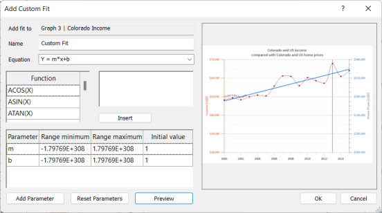
Use the Add Custom Fit dialog to define and add a custom fit curve. |
Defining Custom Fits
To define a custom fit:
- Type the name of the custom fit into the Name field.
- Type the fit equation, using mathematical functions, into the Equation field. For example, a fourth degree polynomial fit would be written as:

This equation is entered into the Equation field as:
Y=a+b*X+c*X^2+d*X^3
If necessary, select a function from the Function list and click Insert to add one of the predefined mathematical functions. You can also double-click a function in the Function list to add it to the Equation field.
Equation parameters should be represented by a single letter, except "x" and "y" which are reserved for the equation variables. Equation parameters are automatically added to the Parameter table as you type the fit equation in the Equation field.
- Review the Parameter table. All parameters in the fit equation should be included automatically. If they are not, check the Equation syntax for errors. If necessary, you can manually add parameters by clicking Add Parameter. Rename added parameters by typing in the Parameter column.
- If you wish to force a range of acceptable values on the parameters, type the minimum acceptable value in the Range minimum column and type the maximum acceptable value in the Range maximum column. This is useful for ensuring Grapher finds the best fit when the parameters are subject to real-life limits imposed by the data being fitted.
- If you have an initial guess for the parameter value(s), set the parameter Initial value by typing in the Initial value column. This is useful for ensuring Grapher finds the global best fit when the Equation is susceptible to local best fit values.
- Optionally, click Preview to preview the custom fit curve. Once a preview is created, you must click Preview again after making changes to the Equation field or Parameter table to update the custom fit preview. If necessary, click Reset Parameters to reset the Parameter table to its default state.
- Click OK to add the custom fit to the graph.
The new custom fit will be available in the Fit type list for all fit curves in the Property Manager on the Plot tab. The custom fit curve is also available by clicking the down arrow under Graph Tools | Add to Graph | Custom Fit.
Editing a Custom Fit Used in a Plot
To edit a fit that is in use by a plot, select the fit and edit the fit properties in the Property Manager on the Plot tab.
Deleting Custom Fits
To remove a fit from the Fit type list, select the custom fit type and click Remove next to Remove fit from types property in the Property Manager on the Plot tab.
Fits and Polar Type Plots
All fits created for a polar plot need to account for the polar coordinates. In a polar plot’s fit equation, the X value is replaced with the angle value, and the Y value is replaced with the radius value. For example, the linear equation for a line/scatter plot is Y=B*X+A. In a polar plot, the linear equation is Radius = B*(Angle) + A.