Available Fits
The following predefined fits are available in the Available Fits drop-down list.
Linear
The Linear fit displays a straight-line fit through the data.

Log
The Log fit displays a natural logarithmic fit through the data.

Exponential
The Exponential fit displays an exponential fit through the data.

or

Power
The Power fit displays a power fit through the data.

or

Spline Smoothing
Spline smoothing produces a uniform curve that passes through all of the data points, regardless of the spacing of the data points or the tension factor applied to the spline fit. Tension factors range from one to 50. Higher tension factors result in straighter lines between the data points and lower tension factors result in more curvature to the fit line. Spline fits do not extrapolate beyond the maximum or minimum data values displayed for the curve. There is not an equation for the Spline smoothing fit.
Polynomial
The Polynomial regression fit displays a curve based on the equation below. The polynomial degree can be set from zero to 10. A polynomial degree of zero is the average Y value, degree one is a linear fit, degree two is a quadratic fit, degree three is a cubic fit, and degree four is a quadric fit.

Orthogonal Polynomial
The Orthogonal polynomial regression fit is an alternate method for calculating polynomial regressions. The Orthogonal polynomial equation has been converted to "normal" polynomial form, so Y can be calculated from a given X with the equation. Alternatively, Y can be calculated from a given X using the orthogonal factors.
Through Origin
The linear fit through the origin forces the linear fit line through the origin (0,0).

Running Average
Running average fits, also called moving average, are generated by taking the average of the data within a specified range on either side of a given point. The window width controls the range of data used in the calculation, and this number must be an odd number between 3 and 1001. For example, the default Window width of 5 averages the data point, the two values above the data point, and the two values below the point. The average of all five values is plotted as part of the fit line. The fit line connects all the average points. The Running average is truncated short of the data limits by a factor of (Window Width - 1)/2 so the fit does not extend to the limits of the plotted data curve.
Weighted Average
The Weighted average fit is similar to the Running average fit. Instead of averaging the points in the Window width equally, a weight is provided for each of the data points (Order) within the window. In a running average fit, all of the weights are equal to one. Therefore, the weighted average fit should provide the same fit as the running average fit if all of the weights are set to one.
LOESS (LOWESS)
The LOESS (LOWESS) fit method fits simple polynomial models to localized subsets of the data. The LOESS (LOWESS) fit is defined by the Span, Family, and Degree. The Span is the proportion of the data used to fit the local polynomial at each point. The Span can vary between 0.1 (10%) and 1.0 (100%) of the data. Typically values between 0.25 and 0.5 are appropriate for the Span parameter. The Span is sometimes referred to as the smoothing parameter. The Family option determines the fit algorithm. When Family is set to Gaussian, a least squares fit is used. A redescending M estimator with Tukey's biweight or bisquare function is used to fit the data when Family is set to Symmetric. The Degree specifies the order of the local polynomials fit to each subset of the data. A Degree of 1 (Linear) fits a linear function to each data subset. A Degree of 2 (Quadratic) fits a quadratic function to each data subset.
See Cleveland, W.S. (1979) "Robust Locally Weighted Regression and Smoothing Scatterplots," Journal of the American Statistical Association, Vol. 74, pp. 829-836. for more information about the LOESS fit.
RMA (Reduced Major Axis)
The RMA fit method fits a linear regression model to the data by minimizing the sum of squares of the perpendicular distance between each data point and the regression line. The RMA method is different from the Linear fit, as the Linear fit uses the ordinary least squares method to minimize the sum of squares of the residuals, i.e. the vertical distance between the data points and the regression line. The RMA fit method is a common method for handling variability in both x and y.
Normal Distribution (Gaussian)
The Normal distribution fit is used with Histograms and 3D Histograms.

Lognormal Distribution
The Lognormal distribution fit is used with Histograms and 3D Histograms.
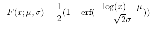
m = scale parameter, s = shape parameter
m, s > 0
erf = standard error function
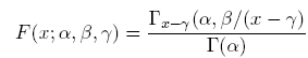
Exponential Distribution
The Exponential distribution fit is used with Histograms and 3D Histograms.
![]()
q = location parameter, s = scale parameter
x³q, and s > 0
Power Distribution
The Power distribution fit is used with Histograms and 3D Histograms.
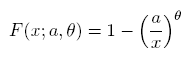
q = shape parameter, a = location parameter
q > 0, and a > 0
Inverse Gaussian Distribution
The Inverse Gaussian distribution fit is used with Histograms and 3D Histograms.
a= shape parameter, b= scale parameter