Orthogonal Polynomial Regression

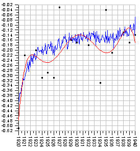
Orthogonal polynomial regression is appropriate and sometimes necessary for higher order polynomial fits, i.e., five degrees and higher. Orthogonal polynomial regression can be used in place of polynomial regression at any time. In the graphic below, the blue curve is a sixth degree polynomial regression and the red curve is a sixth degree orthogonal polynomial regression. Unstable polynomial regressions of this sort can result from round off and truncation errors in the computer arithmetic. The result is a "squiggly" fit line. If the resulting polynomial coefficients are extremely large, relatively small Y values cannot be accurately calculated. Use orthogonal polynomial regression if the polynomial regression oscillates excessively, such as the blue line in the graphic below, or when Y values calculated from the polynomial equation are not approximating the fit curve closely enough.

$image\POLYNOM.png$

Statistics

The orthogonal polynomial regression statistics contain some standard statistics such as a fit equation, polynomial degrees (changed with fit plot properties), and the number of data points used as well as some statistics specific to the orthogonal polynomial such as B[n], Alpha[n], and Beta[n].

Polynomial Factors

Since this is an orthogonal method of calculating the polynomial regression, each degree’s orthogonal polynomial factors are independent of each other. The degree zero results are the optimal zero order fit, the degree one results are the optimal first order fit, and so on. Adding more degrees to the fit does not change the previous degrees’ orthogonal polynomial factors. For example, if a fourth degree orthogonal polynomial regression is calculated from a data set and a separate eighth degree orthogonal polynomial regression is calculated from the same data set, the orthogonal polynomial factors will be the same for degrees zero through four in both statistics results.

Coefficient of Determination

The residual sum of squares and the coefficient of determination (R2) are given for each polynomial degree. The R2 values may be used to indicate when adding degrees do not significantly improve the fit. An R2 value of zero means that no data variation is explained by the orthogonal polynomial degree and an R2 value of one means that all of the data variation is explained by an orthogonal polynomial degree.

Orthogonal Factors

There are two options for calculating Y from a given X with the orthogonal polynomial regression statistics. The simplest method is to use the equation provided in the fit statistics. The orthogonal polynomial factors have been converted to polynomial regression equation coefficients, so that Y can be calculated from X. Alternatively, Y can be calculated from X by using the orthogonal factors: X shift, X scale, B[k], a[k], and b[k].

$image\ortho1.png$

where:

X = XScale*(X-XShift)

k = n, n-1,...,0 where: n is the polynomial degree

Y[n+1] and Y[n+2] = 0 where: n is the polynomial degree

The original X value is scaled before using it in the equation. The highest order equation is calculated first, then the results from that equation are used in the next lower order equation, and so on, until the zero degree equation is solved.

Example

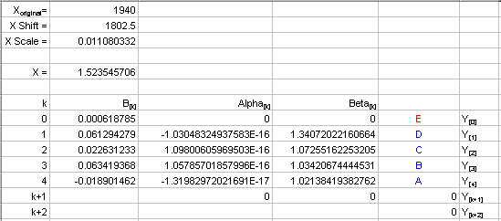
The orthogonal polynomial regression was used as a fit on a data set. X shift, X scale, B[k], a[k], and b[k] are reported in the fit statistics. In this example, Y is calculated for X = 1940. The following table shows the resulting orthogonal factors for a fourth degree orthogonal polynomial regression:

$image\ORTHOONE.png$

To begin calculating Y, first adjust the X value with the X shift and X scale values:

$image\ortho2.png$

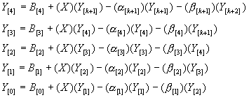
The solution for Y is found by solving the equation below recursively, starting from the highest order (A) and working toward the lowest order (E).

$image\ortho3.png$

where:

X = XScale*(X-XShift)

k = n, n-1,...,0 where: n is the polynomial degree

Y[n+1] and Y[n+2] = 0 where: n is the polynomial degree

The following are the equations for solving for Y given 1940 as X (remember that the adjusted X is used in the equation):

$image\ortho4.png$

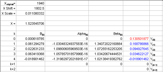
The results for Y[n] are shown in blue and red in the following table. Given X=1940, Y=0.13 (Y[0]).

$image\ORTHOTBL.png$